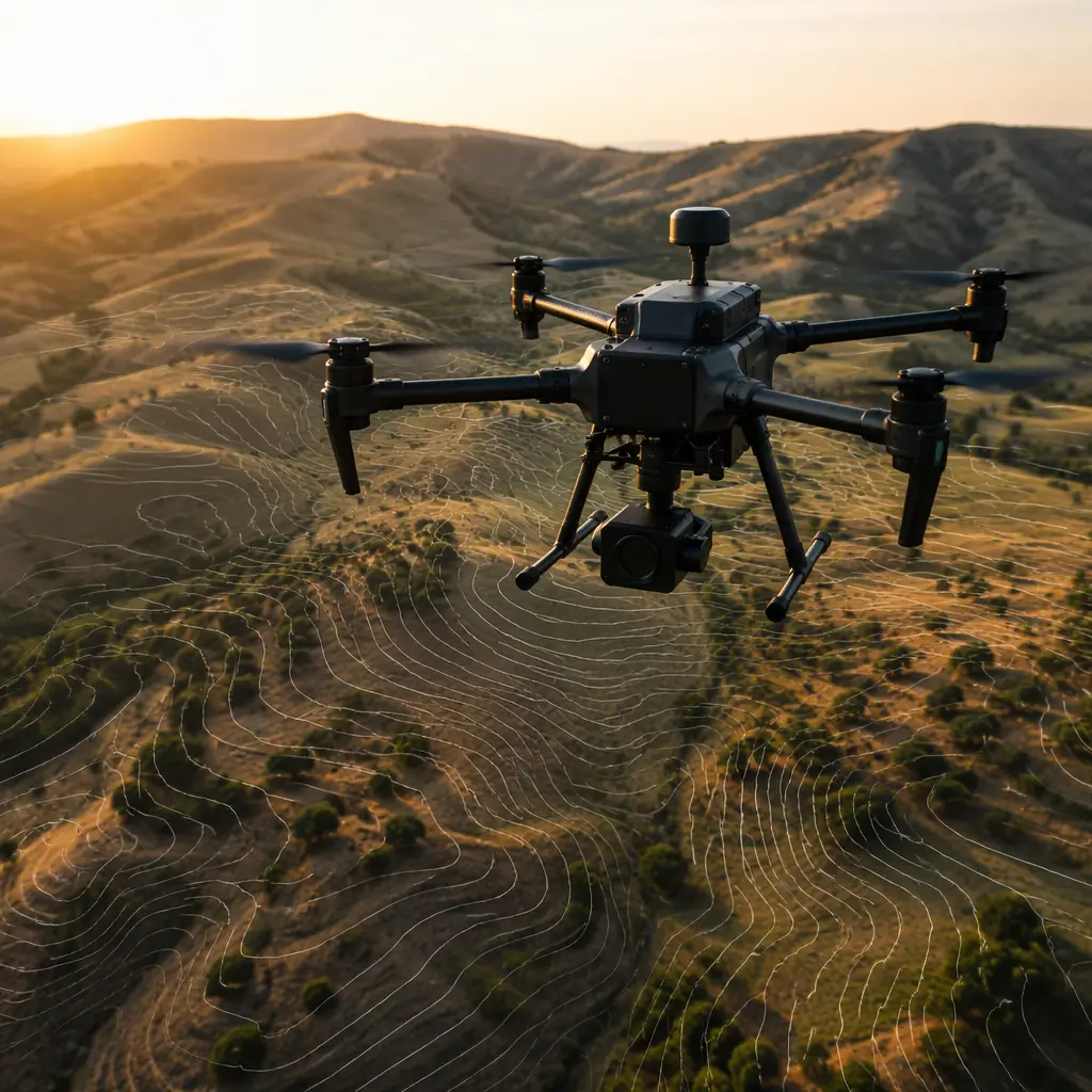
Aerial mapping with UAVs has transformed from a niche surveying technique to a mainstream data acquisition method. The global UAV mapping market crossed USD 3.8 billion in 2025, with survey-grade photogrammetry and LiDAR platforms representing the fastest-growing segment at 18.7% CAGR. But the component supply chain for mapping drones is fundamentally different from the general UAV market — the components that make a drone fly are not the same components that make a drone produce survey-grade data. Understanding which specifications matter for geospatial accuracy, and which are irrelevant marketing numbers, is the difference between delivering a 2 cm GSD orthomosaic that passes a client's accuracy audit and delivering imagery that requires three rounds of ground control point correction.
The mapping drone component chain has four links, and accuracy degrades at every link that is underspecified. The GNSS receiver determines where each image was captured. The camera or LiDAR sensor determines what was captured. The airframe and flight controller determine the stability of the platform during capture. And the data link determines whether the operator can monitor data quality in real time or discovers a focus error after landing. A weakness in any one link propagates through the entire geospatial pipeline — a precise GNSS receiver paired with a consumer-grade camera on an unstable airframe produces precisely geo-located unusable imagery.
This article addresses component selection for mapping and survey UAVs from a procurement perspective. It assumes you have already settled the foundational system architecture questions discussed in the UAV supply chain layers framework and are now selecting specific components for a mapping platform. The guidance covers both photogrammetry platforms (camera-based, the most common configuration) and LiDAR platforms (for terrain modeling under vegetation canopy), with the component trade-offs specific to each.
GNSS receivers: the foundation of survey accuracy
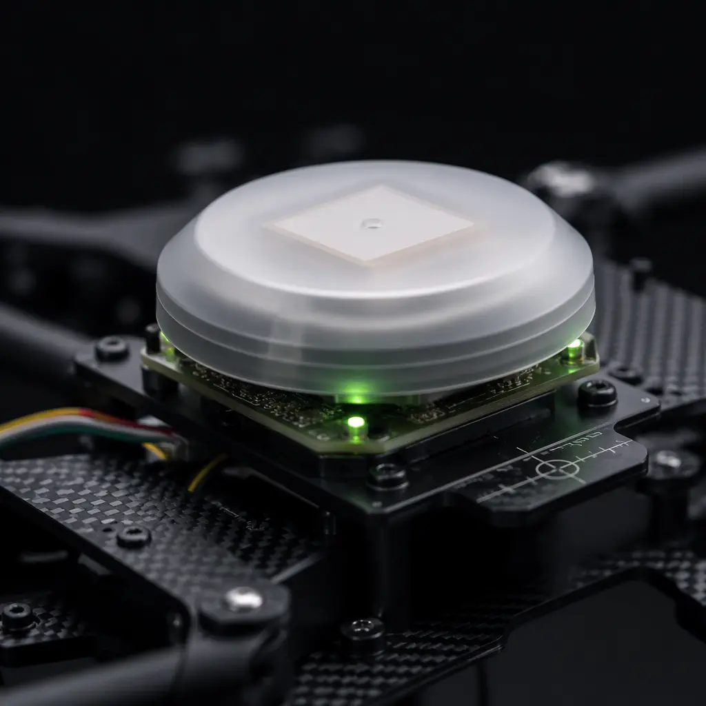
In a mapping drone, the GNSS receiver is not a navigation accessory — it is the primary measurement instrument. Every image in a photogrammetry dataset is positioned by the GNSS receiver's output at the moment of exposure. A GNSS error of 2 meters at the receiver translates to a 2-meter error in the georeferenced orthomosaic, regardless of the camera's optical quality or the flight controller's stability. For survey-grade work, the GNSS receiver must deliver centimeter-level accuracy in real time, and it must timestamp each position fix with sufficient precision to align with the camera's exposure events.
The minimum configuration for survey-grade mapping is a multi-band (L1/L2 or L1/L5) GNSS receiver with RTK correction input, delivering horizontal accuracy of 1 cm + 1 ppm and vertical accuracy of 2 cm + 1 ppm when receiving corrections from a local base station or an NTRIP (Networked Transport of RTCM via Internet Protocol) caster. The u-blox F9P module — the de facto standard for UAV mapping receivers — achieves these specifications with a 10 Hz position update rate and 20 ns timestamp resolution. At 10 m/s flight speed (36 km/h), a 10 Hz update rate captures one position every 1 meter of forward travel, which is adequate for mapping GSD (ground sample distance) down to approximately 2 cm. For higher-resolution mapping at 1 cm GSD flying at 5 m/s, consider a receiver with 20 Hz update rate to maintain the 1-position-per-25 cm sampling density.
The RTK correction link deserves as much attention as the receiver itself. A mapping drone operating 5 km from the base station in rolling terrain may lose the RTK correction radio link if the base station antenna is not elevated above ground clutter. The correction data link architecture has three tiers: a dedicated 868/915 MHz radio link from the base station to the aircraft (most reliable, requires line of sight), an NTRIP connection over the aircraft's 4G/LTE modem (convenient but dependent on cellular coverage at altitude), or PPK (post-processed kinematic) recording with no real-time correction link at all — the receiver logs raw observations and corrections are applied after the flight. PPK eliminates the correction link as a failure point but removes the operator's ability to verify positioning accuracy during the mission. For the RF fundamentals of the radio link, see the UAV RF communication systems guide.
 Concept illustration
Camera selection for photogrammetry
The camera on a mapping drone is not judged by its video capabilities, its autofocus speed or its low-light performance. It is judged by three specifications: sensor resolution (megapixels), lens distortion characteristics, and the mechanical stability of the lens mount relative to the sensor plane. These three parameters determine the achievable GSD, the geometric accuracy of the photogrammetric reconstruction, and the repeatability of the camera calibration between flights.
Sensor resolution and GSD. The ground sample distance — the physical distance on the ground represented by one pixel — is calculated as GSD = (sensor pixel size × flight altitude) / focal length. For a Sony A7R IV (61 MP full-frame, 3.76 μm pixel pitch) with a 35 mm lens flying at 120 m AGL: GSD = (3.76 μm × 120 m) / 35 mm = 1.29 cm. For a DJI P1 (45 MP full-frame, 4.4 μm pixel pitch, 35 mm lens) at the same altitude: GSD = (4.4 μm × 120 m) / 35 mm = 1.51 cm. The difference between 1.29 cm and 1.51 cm GSD does not matter for most topographic surveys — both are well below the 5 cm threshold required for 1:500 scale mapping — but it matters for volumetric measurement of stockpiles where a 0.22 cm GSD difference across a 10,000 m² site compounds to approximately 22 m³ of volume uncertainty.
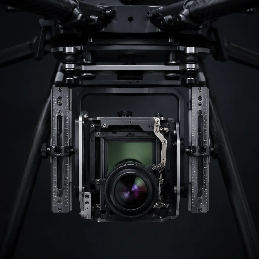
Lens distortion and calibration. Every lens introduces radial and tangential distortion that shifts pixel positions from their ideal locations. Photogrammetry software (Pix4D, Agisoft Metashape, RealityCapture) corrects for this distortion using a camera calibration model, but the calibration is only as good as the stability of the lens mount. A lens that shifts by 0.01 mm in its mount between flights — from thermal expansion, vibration or focus motor preload — changes the principal point location and introduces systematic error that the calibration model from the previous flight does not capture. The solution is a fixed-focus lens with a locked focus ring (set to infinity or the hyperfocal distance for the mapping altitude, typically 30–50 m for most survey configurations) and a rigid lens mount — ideally a screw-lock or flange-mount system rather than a bayonet mount, which has 20–50 μm of mechanical play.
Mechanical shutter vs. electronic rolling shutter. A mechanical shutter exposes the entire sensor simultaneously, producing an image where every pixel represents the same instant in time. An electronic rolling shutter exposes the sensor line by line, typically taking 1/15 to 1/30 second to scan the full frame. At 10 m/s flight speed, a rolling shutter that takes 1/20 second to scan produces a 0.5-meter displacement between the first and last pixel row — geometric distortion that photogrammetry software models as a combination of camera tilt and translation, introducing systematic error into the bundle adjustment. For survey-grade work, a camera with a mechanical shutter and global flash sync output (to trigger the GNSS receiver's event marker with microsecond precision) is non-negotiable. Cameras without a mechanical shutter can still be used for non-survey mapping at GSD above 3 cm, where the rolling shutter distortion is smaller than the GSD and the photogrammetry software's self-calibration absorbs the residual error.
 Concept illustration
LiDAR payloads for terrain modeling and vegetation penetration
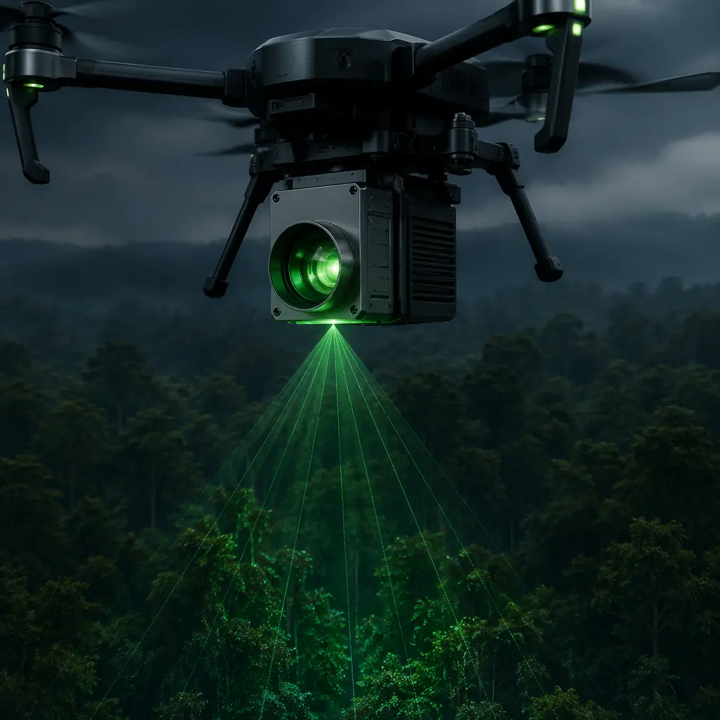
Photogrammetry produces excellent surface models of bare earth, buildings and infrastructure — but it cannot see through vegetation. A forested site, a construction area with tall grass, or a power line corridor with tree canopy all require LiDAR to capture the ground surface beneath the vegetation. The laser pulses penetrate gaps in the foliage and record multiple returns per pulse; the last return is assumed to represent the ground surface, while intermediate returns represent vegetation structure.
A survey-grade UAV LiDAR system consists of a laser scanner, an IMU (inertial measurement unit) and a GNSS receiver, all rigidly mounted on a common baseplate with precisely known lever-arm offsets between each component's reference point. The laser scanner specifications that matter for mapping are pulse repetition frequency (PRF), maximum returns per pulse, and range accuracy at the target reflectance. A scanner with 200 kHz PRF and dual-return capability produces 400,000 points per second — enough for a point density of 200–400 points/m² at 60 m AGL flying at 5–6 m/s, which is adequate for 1:500 scale topographic mapping and engineering design. Triple-return or quad-return scanners (600 kHz PRF, up to 4 returns per pulse) push point density to 500–800 points/m² under canopy, sufficient for detecting fine terrain features like drainage channels and erosion rills.
The IMU is the limiting component in a UAV LiDAR system, not the laser. A laser scanner with 2 cm range accuracy paired with an IMU that drifts 0.05° per minute produces a position error of tan(0.05°) × 60 m = 5.2 cm at the target — more than double the laser's inherent accuracy. A survey-grade IMU for UAV LiDAR, such as the Applanix APX-15 or the KVH 1750, achieves 0.02–0.03° roll/pitch accuracy and 0.08–0.10° heading accuracy with post-processed tightly-coupled GNSS/IMU integration. This class of IMU adds approximately USD 8,000–15,000 to the payload cost but is the difference between a point cloud that passes an engineering accuracy audit and one that requires ground truth correction at every control point.
The weight budget for a LiDAR payload is tight: a complete UAV LiDAR system (scanner + IMU + GNSS + baseplate + cabling) weighs 1.2–2.5 kg, representing 15–30% of a mapping drone's payload capacity. Every gram above 2 kg reduces flight endurance by approximately 1.5–2.5 minutes on a typical 12S multirotor platform. The component-level decisions — selecting a scanner with integrated IMU vs. separate components, aluminum vs. carbon fiber baseplate, integrated vs. external GNSS antenna — collectively determine whether the payload is practical for a given airframe. For the mechanical integration considerations, including vibration isolation and CG placement, the UAV payload integration guide covers the mounting and isolation strategy in detail.
 Concept illustration
Airframe configuration for mapping endurance and stability
Mapping missions demand flight endurance above all other performance metrics. A 300-hectare topographic survey at 2 cm GSD requires approximately 45–60 minutes of flight time at 8–10 m/s in a lawnmower pattern with 70% forward overlap and 60% side overlap. This endurance requirement eliminates most multirotor configurations running 6S LiPo batteries — the practical limit for a 6S multirotor carrying a 1.5 kg mapping payload is 25–32 minutes, insufficient for sites larger than approximately 120 hectares in a single flight.
The airframe configuration for mapping has converged on two platforms: large multirotors (hexacopter or octocopter, ≥1,200 mm wheelbase) running 12S Li-Ion battery systems for sites up to 400 hectares, and VTOL fixed-wing hybrid platforms for corridor mapping and sites exceeding 500 hectares where transit distance to the survey area becomes the dominant time component. A 12S hexacopter with 28-inch propellers, 380 KV motors and a 28,000 mAh 12S8P Li-Ion pack achieves 55–65 minutes of mapping endurance with a 1.5 kg payload at 10 m/s cruise — covering approximately 350–400 hectares per flight with conservative overlap settings. The powertrain matching methodology for this configuration is covered in the UAV powertrain matching guide.
Airframe vibration is the hidden enemy of mapping accuracy. A camera mounted on an airframe that vibrates at 80–120 Hz (typical motor/propeller harmonic for 28-inch props at 4,000 RPM) transfers that vibration to the camera's sensor plane. At the sensor level, 5–10 μm of vibration amplitude during a 1/1000 second exposure produces approximately 1–3 pixels of image blur at 3.76 μm pixel pitch — enough to degrade the photogrammetry software's feature-matching accuracy and reduce the effective GSD by 30–50%. The vibration isolation strategy for mapping cameras is different from gimbal isolation: because the camera is rigidly mounted (no gimbal) to maintain the geometric relationship between the camera optical axis and the GNSS antenna phase center, the isolation must be applied between the airframe and the payload mounting plate, not between the payload and the camera. Wire rope isolators tuned to 10–15 Hz natural frequency under the payload mass provide 80–90% vibration attenuation at 80 Hz while maintaining the rigid geometric relationship within the payload assembly. For the structural stiffness considerations that determine isolation effectiveness, see the UAV airframe materials guide.
Flight controller requirements for automated mapping
A mapping drone's flight controller must execute automated survey missions with precise waypoint tracking, consistent ground speed control, and reliable trigger output synchronization with the camera. The ArduPilot and PX4 ecosystems both support automated survey missions — ArduPilot's Auto mode with Survey grid generation and PX4's Mission mode with survey pattern generation — but the flight controller hardware must support the specific interface requirements of the mapping payload.
The critical interface is the camera trigger signal. The flight controller must output a trigger pulse at each exposure point with timing accuracy better than 10 ms relative to the GNSS position fix. At 10 m/s, a 10 ms timing error translates to a 10 cm position error for that image — introducing systematic georeferencing error that varies with flight direction and cannot be modeled as a simple offset. The trigger mechanism options, in order of timing precision: a hardware PWM output with interrupt-driven timing (best, < 1 ms jitter), a relay output driven from a serial command (acceptable, 5–10 ms jitter), or a software-triggered GPIO (worst, 15–50 ms jitter depending on CPU load). For survey-grade work, the hardware PWM trigger with the flight controller's internal hot shoe event logging — which records the exact GNSS timestamp of each trigger pulse — provides the most accurate image georeferencing.
Terrain following is essential for mapping sites with elevation variation. A survey grid flown at a constant barometric altitude over terrain with 50 meters of elevation change produces GSD variation of approximately 40% between the highest and lowest points — images captured at 170 m AGL (over a valley floor) have 42% larger GSD than images captured at 120 m AGL (over a hilltop), creating inconsistent feature resolution that degrades the photogrammetry software's tie-point matching. Terrain following using SRTM or ASTER GDEM elevation data loaded onto the flight controller — with the autopilot adjusting the target altitude at each waypoint based on the terrain elevation beneath it — maintains consistent GSD across the entire site. The flight controller must support terrain following with a digital elevation model (DEM) loaded onto the SD card; ArduPilot's TERRAIN_ENABLE and TERRAIN_FOLLOW parameters activate this feature. For the ESC and motor response requirements that enable precise altitude tracking during terrain following, the flight controller and ESC matching guide covers the protocol and timing constraints.
Procurement checklist: 7 component decisions for mapping drones
These seven component decisions form the minimum validation gate before ordering hardware for a mapping UAV. Each item maps to a specific geospatial accuracy requirement.
1. GNSS receiver configuration. Multi-band L1/L2 or L1/L5 receiver with RTK or PPK capability, ≥10 Hz update rate, event marker input with ≤50 ns timestamp resolution. Validate by logging a static 30-minute position with RTK corrections: the horizontal standard deviation should be ≤1.5 cm and the vertical ≤3 cm. A receiver that achieves 1 cm accuracy on the datasheet but drifts to 5 cm during a ground test will produce systematic georeferencing errors across every image in the survey.
2. Camera and lens combination. Mechanical shutter with global flash sync output, fixed-focus lens with locked focus ring, ≥36 MP full-frame sensor for survey-grade work (or ≥20 MP APS-C for non-survey mapping at > 3 cm GSD). Verify the lens distortion profile is stable: capture 20 images of a calibration target from different angles, process in a photogrammetry software package, and confirm the reprojection error is ≤0.3 pixels. A lens whose distortion parameters change between calibration sessions indicates an unstable mount and will produce systematic error that the bundle adjustment cannot fully model.
3. IMU class for LiDAR payloads. For LiDAR systems: roll/pitch accuracy ≤0.03°, heading accuracy ≤0.10° with post-processed GNSS/IMU integration. Verify that the IMU's gyro bias stability and random walk specifications are appropriate for the expected flight duration — a gyro with 3°/hr bias instability accumulates approximately 0.05° of angular error over 60 minutes, acceptable for most UAV LiDAR surveys.
4. Battery and endurance configuration. 12S or 14S Li-Ion with 21700 cells, targeting ≥50 minutes of mapping endurance at cruise speed with the survey payload. The battery capacity should be derived from a measured power consumption test — not from a manufacturer's endurance estimate — with the aircraft configured exactly as it will fly the survey mission, including the payload drawing full operational power. The cell-level details of Li-Ion pack configuration, BMS requirements and thermal management are covered in the UAV battery and power management guide.
5. Propeller and motor matching for endurance cruise. Large-diameter, low-pitch propellers (24–28 inch, 5.5–7.0 inch pitch) with low-KV motors (100–180 KV at 12S) optimized for the mapping cruise speed of 8–12 m/s, not for hover efficiency. At cruise speed, the propellers operate in translational lift with 15–25% higher aerodynamic efficiency than in hover — the motor and propeller combination should be selected for the cruise operating point, not the hover operating point. The full matching chain from voltage through ESC to propeller load is detailed in the powertrain matching guide.
6. Vibration isolation for rigid-mount cameras. Wire rope or silicone gel isolators between the airframe and the payload mounting plate, tuned to 10–15 Hz natural frequency under the full payload mass. Validate with an accelerometer mounted at the camera's sensor plane during a full-throttle sweep: vibration amplitude at the sensor should be below the pixel pitch of the camera (3.76 μm for a 61 MP full-frame sensor) across the full throttle range.
7. Terrain following capability. Flight controller with terrain following using a digital elevation model, maintaining ±5 m altitude accuracy relative to the loaded DEM. Validate by flying a survey grid over terrain with 30+ meters of elevation variation and checking that the GSD variation across the site is within ±10% — if GSD varies by more than ±15%, the terrain following parameters or the DEM resolution need adjustment.
For teams evaluating whether to build a custom mapping platform from individual components or procure a pre-integrated system, the cost-benefit framework in the UAV component build vs. buy guide provides a structured decision process across the three sourcing depths.
Explore mapping solutions Back to Blog
Continue Reading
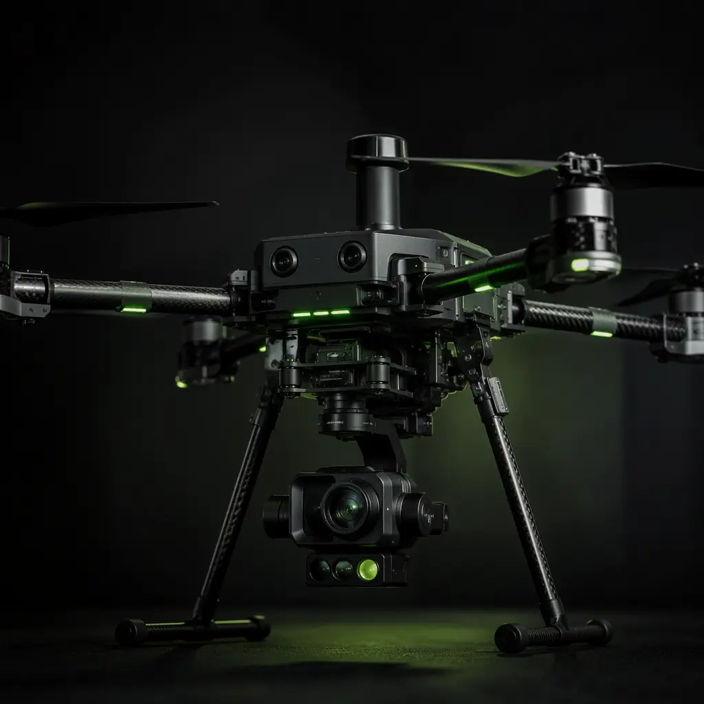
UAV Payload Integration Guide
Mounting, vibration isolation and CG management for mapping sensors.
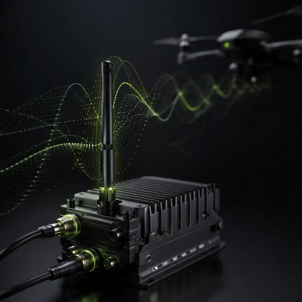
UAV RF Communication Systems
RTK correction links and telemetry coordination for long-range survey.
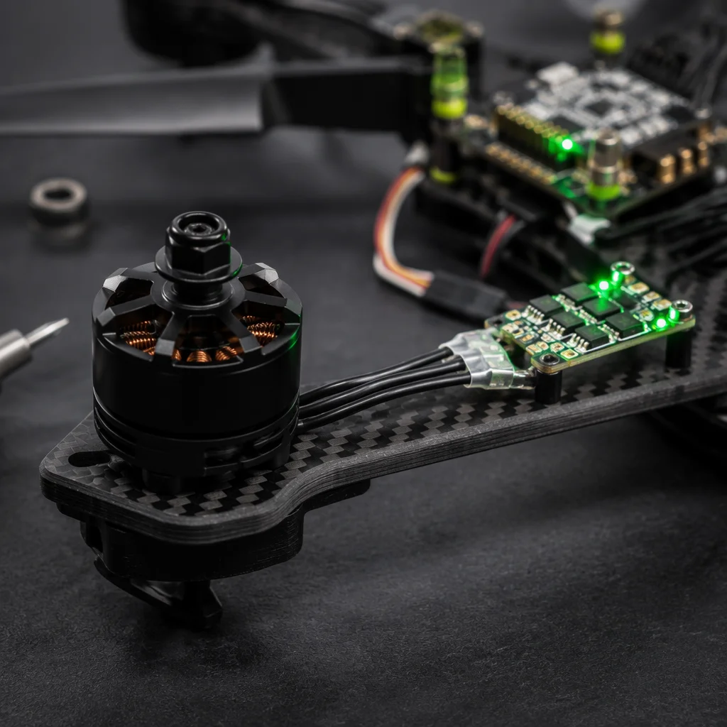
UAV Powertrain Matching
Motor KV, propeller sizing and ESC selection for mapping cruise efficiency.
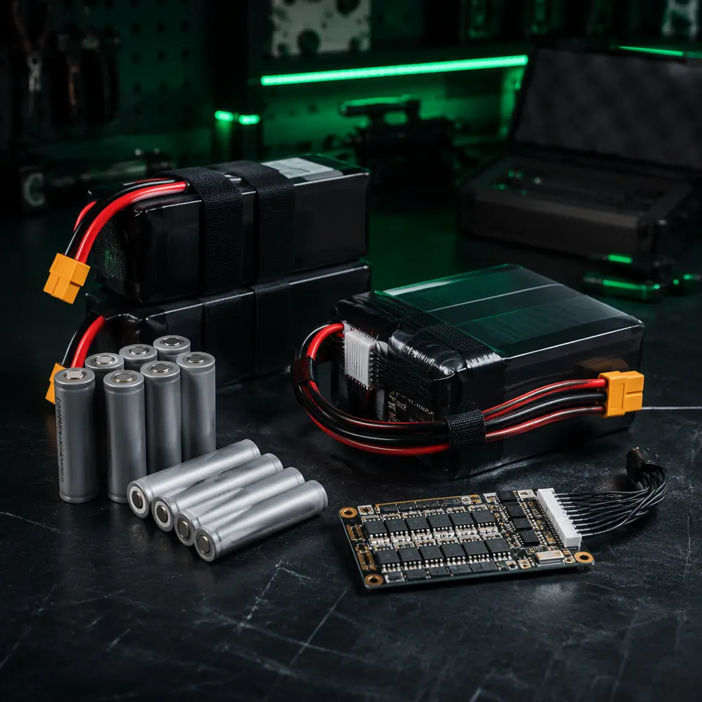
Battery & Power Management
12S Li-Ion pack configuration for 50+ minute mapping endurance.
Airframe Materials Guide
Structural stiffness requirements for vibration-free mapping sensor mounting.